We have covered the features behind the hours prices in the EDA post (link.) In this post, we will use a classic (statistical) Machine Learning technique – Multiple Regression – to predict the prices.

First, let’s load the necessary packages and create the theme for the charts.

The train dataset contains 81 features that can be utilized for machine learning except ‘Id.’ So I’ll just get rid of it and also set up a new dataset.

One interesting thing about this dataset is that there are many categorical variables with NAs. Let’s see…

We know that there are 1453 NAs in PoolQC feature. How many valid datadpoints does PoolQC have?

So, there are only seven valid data points: 2Ex, 2Fa, and 3Gd.

We sure can get rid of the feature altogether as it seems like the majority of the data doesn’t have a pool. But what if having a pool is statistically significant? Also, not to mention that many other features might be in the same situation as PoolQC.

So, here is what we are going to do. We will add “None” as another level in the factor variable.

The code will loop through every feature and see if it is a factor variable. If yes, it will change from NA to “None” which will be treated as another legitimate level.

Now let’s see again if we have any NA.

Oh okay, there are still some NAs. But where are they from?

Okay, so it is from LotFrontage, MasVnrArea, and Garage Year Built. Those two are easy enough. According to the definition, LotFrontage is Linear feet of street connected to the property. If it is NA, that means a property is not connected to the street. So, I’ll just change it to zero. As for MasVnrArea, its definition is Masonry veneer area in square feet. If it is NA, that means it is 0. So for these two, I’ll just change from NA to zero.

We still have GarageYrBlt. Hmm, This one is interesting. It is numeric and those with 0 likely means they don’t have a garage. We could also convert the feature to factor variable, but when we run the regression, yikes, there will be ten plus features, and if they were to be significant, we could kiss goodbye to our dear parsimony. Therefore, in this case, I’ll just drop GarageYrBlt. 🙂

Next, I’ll split them to train and test sets.

Alright, let’s start by building the models using Forward, Both, and Stepwise.

It is going to take some time depending on the CPU power. Let’s take a look at AIC which measures the complexity of the model.

We can see that Stepwise and Backward methods’ AICs are pretty close 23,511 and 23,512. Next, let’s take a look at RMSE.

Again, Stepwise’s and Backward’s RMSEs are close again. What about Adjusted R-Square and overall fit of the models?

I’ll show only a portion of the results.

I mean, seriously, they aren’t that different. What we should do next is to take a look at various plots, but to make things easier I’ll just do one which is Stepwise.

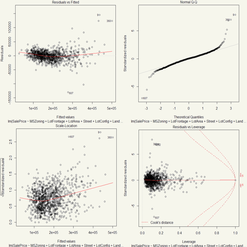
Well, they are mostly quite okay. Most of the points in QQ Plot are on the diagonal line. Most of the data points have small Cook’s D. Heteroscedasticity is quite held as the shape is quite even.

The plot()  function has done a great job giving us the essential charts. But I’d like to see the leverage in another form.

Yeah, well, that is surely a whole lot of leverage points with value 1. That’s high! We sure can make it better. It is clear that there are outliers and high leverage data points in the dataset. I could chop them off. But I’ll employ log transformation.

Alright, let’s see the diagnostics.

Hm, 0.9436 Adjusted R-Squared, significant p-value, and -1945.451 AIC. That was a huge improvement. Let’s summarize the diagnostics from our four different models.

But one thing that stands out to me is 167 features. Ugh… They are bloated because many of them are factor variables. So, next improvement is to get rid of those that are not statistically significant. Luckily, R distinguishes that by the asterisk. So, I’ll just remove statistically insignificant features in the next model.

Alright, let’s see the stats again.

Okay, now it gets much less complicated! All Hail Parsimony!!! Ah, but that comes with a cost. RMSE is almost twice that of Stepwise_log model and adjusted R-square, for the first time, is below 0.90.

For now, I’d choose Stepwise_log_2 model. Now, let’s see the charts.

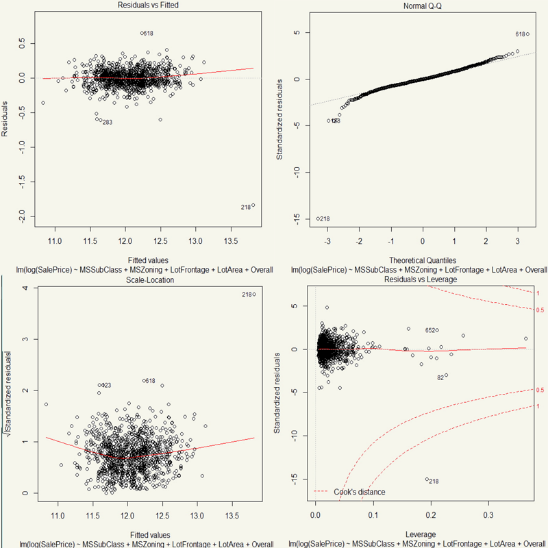
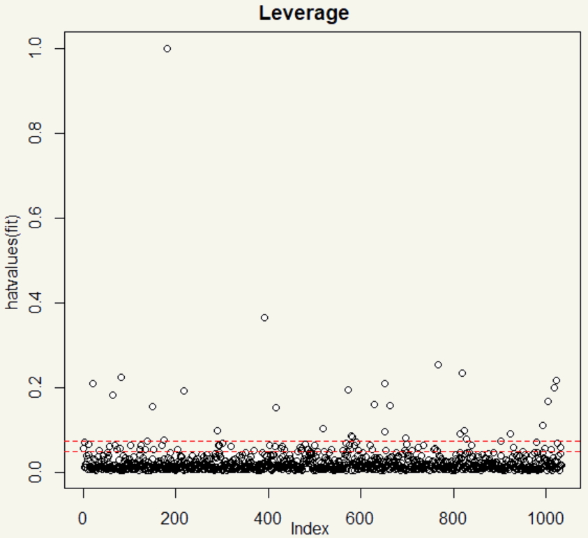
Nice. We did reduce the leverage point by, well, almost all by just simply taking a log. But still, there are a number of those leverage points around.
You know what, I’ll just run another model with the same features but excluding those leverage points.

Let’s see the stats.

Okay, that’s good. Those leverage points distorted our prediction. Up to this point, there are six models.

In term of Adjusted R-Square and RMSE, in my opinion, they aren’t that different. But they are significantly different, in term of parsimony. I mean, 240 features!?

And so it now comes down to the good old question: Predictive power or Parsimony?

I chose parsimony for Stepwise_log_3. 😊 Think about it in a different angle.

Comparing Stepwise_log_3’s 0.89 Adjusted R-Square to that of model 1 (0.93), it is only 0.04 apart. But the reduction in the number of features is 216. Well, for me, Stepwise_log_3 is the winner.

Now that we got our model, we need to make a real prediction on the test set. I’ll add them back to the test set for charts.

Let’s see how they look.

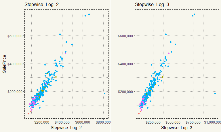
They are not that different at all, right? The overall shape is essentially the same. The difference is the outlier on the right in which Stepwise_Log_2 model forecasted $800,000, but Stepwise_Log_3 model predicted $1,000,000. I’d guess Stepwise_Log_3’s RMSE is more than that of Stepwise_Log_2.

Yep. No doubt. But I’m just curious, what would the delta look like if we were to exclude the outliers.

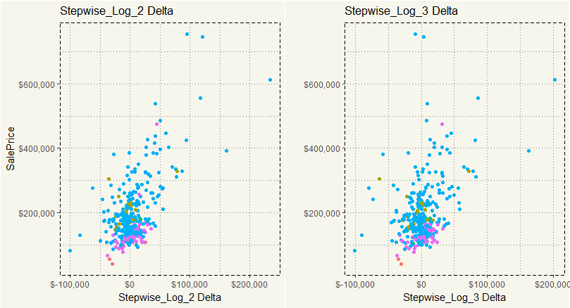
Yep, that is about the same.

TL;DR: Multiple Regression works well for predicting house prices. However, the tradeoff of parsimony and predictive accuracy exists. In this case, I chose parsimony.