In this tutorial, we will cover another popular Tree-based Machine Learning technique: Conditional Inference Tree (CIT.)
We will apply CIT on HR dataset published in Kaggle (here).
One significant difference for CDT and Classical Decision Tree is the use of p-value as one a split criterion instead of using homogeneity. The algorithm will pick the feature with the least p-value and will start splitting from it. Then it will keep going until it no longer finds statistically significant p-value or some other criteria have met such as minimum node size or max split. We left off last time with the conclusion that Classical Decision Tree did not use any categorical variable to do the split. Let’s see if CDT will do the same.
First, let’s load data and necessary packages. We will need “partykit” package for CIT.
|
1 2 3 4 5 6 |
##### Load Packages ##### library(dplyr) library(partykit) ##### Load Data ##### data <- read.csv("C:/Users/data.csv", stringsAsFactors = T) |
Before we can do anything, we need to do one-hot encoding and changing some column names.
|
1 2 3 4 5 6 7 8 9 10 11 12 13 14 15 16 17 18 19 20 |
##### One-Hot Encoding ##### ml <- data %>% rename(department = sales, accident = Work_accident, avg_mth_hrs = average_montly_hours, tenure = time_spend_company, promotions = promotion_last_5years) %>% mutate(dep_hr = ifelse(department == "hr", 1,0)) %>% mutate(dep_IT = ifelse(department == "IT", 1,0)) %>% mutate(dep_mngt = ifelse(department == "management", 1,0)) %>% mutate(dep_mkt = ifelse(department == "marketing", 1,0)) %>% mutate(dep_prod = ifelse(department == "product_mng", 1,0)) %>% mutate(dep_RandD = ifelse(department == "RandD", 1,0)) %>% mutate(dep_sales = ifelse(department == "sales", 1,0)) %>% mutate(dep_sup = ifelse(department == "support", 1,0)) %>% mutate(dep_tech = ifelse(department == "technical", 1,0)) %>% mutate(sal_med = ifelse(salary == "medium",1,0)) %>% mutate(sal_high = ifelse(salary == "high",1,0)) %>% #removing original variables select(-department, -salary) |
Next, we split them into train and test sets.
|
1 2 3 4 5 6 7 |
##### Train & Test Sets ##### size <- floor(0.75*nrow(ml)) set.seed(999) train_index <- sample(seq_len(nrow(ml)), size = size) train <- ml[train_index,] test <- ml[-train_index,] |
Now is the time to build the model.
|
1 2 |
##### Conditional Tree - Train ##### tree <- ctree(left~., data = train, control = ctree_control(mincriterion = 0.70)) |
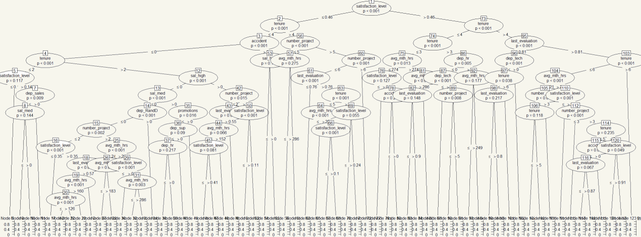
Mincriterion controls the significance parameter. I set it to unusually low to demonstrate the effect of the effect on the feature selection. Before I create the tree, do you think what factor has the lowest p-value?
|
1 |
plot(tree) |

Whoa… that’s huge. There are many variables included in the tree. Surely, categorical variables are included! The highest node is… Satisfaction_Level! I realized that the chart is somewhat… incomprehensible as there are so many details in there. Unfortunately, the “partykit” package doesn’t give that much flexibility to configure the charts. There are some workarounds on the Internet, but they were not so helpful in this case. So I just kept it as it was with some help from GIMP to change the background color.
Now, it is the time to see if that super complicated tree will give good predictive power.
|
1 2 3 4 5 |
##### Predict ##### ctree.pred <- round(predict(tree, test, type="response")) ##### Confusion Matrix ##### table(test$left, ctree.pred, dnn=c("Actual", "Predicted")) |
|
1 2 3 4 5 |
> table(test$left, ctree.pred, dnn=c("Actual", "Predicted")) Predicted Actual 0 1 0 2768 99 1 111 772 |
\(\frac{2768+772}{3750}=94.4\%\) That’s not bad at all.
But come to think about it, 70% confidence level is too low. There could be features that are not statistically significant yet included in the model. Let’s increase mincriterion to 0.95 or 95% Confidence Level.
|
1 2 3 4 5 |
##### 95% Confidence Level Train ##### tree2 <- ctree(left~., data = train, control = ctree_control(mincriterion = 0.95)) ##### Plot ##### plot(tree2) |

Oh, that is less complex, although not that much. Let’s see its predictive power.
|
1 2 3 4 5 |
##### Predict ##### ctree.pred2 <- round(predict(tree2, test, type="response")) ##### Confusion Matrix ##### table(test$left, ctree.pred2, dnn=c("Actual", "Predicted")) |
|
1 2 3 4 5 6 |
##### Confusion Matrix ##### > table(test$left, ctree.pred2, dnn=c("Actual", "Predicted")) Predicted Actual 0 1 0 2773 94 1 114 769 |
The accuracy is \(\frac{2773+769}{3750} = 94.5\%\) It is just a little improvement over 70% confidence. Regardless, this is a pretty good bang for the buck Machine Learning technique as it yields over 90% accuracy with very minimal time to execute!
TL;DR: In the HR Dataset, Conditional Inference Tree could not yield a better result that Classical Decision Tree. However, both gives over 90% accuracy with less than 3 seconds to execute. Tree is surely an excellent tool you may want to consider.
