Lasso Regression is another method in improving a model through adjusting coefficients. Unlike Ridge Regression in which every variable is still kept in the model, Lasso Regression could create a model with only a subset of all variables.
Lasso penalty term is as follows:
$$\lambda\sum_{j=1}^p|{\beta_{j}|}$$
We need to come up the value of \(\lambda\) as in Ridge Regression. So, let’s get started.
|
1 2 3 4 5 6 7 8 9 10 11 12 13 14 15 16 17 |
##### Load Goodies ##### library(tidyverse) library(glmnet) library(gridExtra) ##### Theme ##### theme_moma <- function(base_size = 12, base_family = "Helvetica") { theme( plot.background = element_rect(fill = "#F7F6ED"), legend.key = element_rect(fill = "#F7F6ED"), legend.background = element_rect(fill = "#F7F6ED"), panel.background = element_rect(fill = "#F7F6ED"), panel.border = element_rect(colour = "black", fill = NA, linetype = "dashed"), panel.grid.minor = element_line(colour = "#7F7F7F", linetype = "dotted"), panel.grid.major = element_line(colour = "#7F7F7F", linetype = "dotted") ) } |
|
1 2 3 |
#### Check NAs ##### data <- mtcars sum(is.na(data)) |
|
1 2 |
> sum(is.na(data)) [1] 0 |
We will use the glmnet library and mtcars dataset. We need to create a matrix of predictors as a data frame is not applicable to glmnet() .
|
1 2 |
##### Create a data ###### web_x <- model.matrix(mpg ~ ., data)[,-1] |
Next, we create an array of the dependent variable.
|
1 2 |
##### Creating Y ##### web_y <- data$mpg |
Then we separate 80% of data to a training set, 20% to a test set.
|
1 2 3 4 5 |
##### Splitting Train and Test Sets ##### train_number <- round(0.8*nrow(data),digit=0) set.seed(999) train_index <- sample(seq_len(nrow(data)), size = train_number) test_index <- (-train_index) |
Now we are ready to fit the Lasso Regression. First, we will use automatic \(\lambda\) generation from glmnet() .
|
1 2 3 4 5 |
##### Fit Lasso ##### lasso <- glmnet(x[train_index,], y[train_index], alpha = 1, thresh = 1e-12,nlambda=100) |
Then a for loop() for MSE calculation.
|
1 2 3 4 5 6 7 8 9 10 |
MSE <- rep(0,100) for (i in 1:100){ ridge.pred <- predict(lasso, s=lasso$lambda[i], # s= lambda_range, newx = x[test_index,]) print(lasso$lambda[i]) # print(ridge.pred) MSE[i] <- mean((ridge.pred - y[test_index])^2) } |
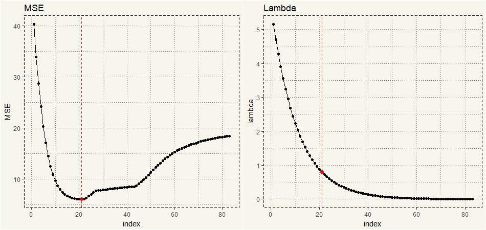
Here is the lowest MSE.
|
1 2 3 |
##### Min MSE ##### min_mse <- min(MSE) min_mse |
|
1 2 |
> min_mse [1] 6.130318 |
GGPLOT visualization:
|
1 2 3 4 5 6 7 8 9 10 11 12 13 14 15 16 17 18 19 20 21 22 23 24 |
##### Creating Data for Visualization ##### lambda_mse <- data.frame(lambda = lasso$lambda, MSE = MSE, index = c(1:83)) image_mse <- ggplot(lambda_mse,aes(x = index, y = MSE)) + geom_line() + geom_point() + theme_moma() + geom_point(data = subset(lambda_mse, MSE == min_mse), aes(x = index, y = MSE), size = 2, col = 'red') + geom_vline(xintercept = 21, linetype = "dashed", col = 'red') + ggtitle("MSE") image_lambda <- ggplot(lambda_mse,aes(x = index, y = lambda)) + geom_line() + geom_point() + theme_moma() + geom_point(data = subset(lambda_mse, MSE == min_mse), aes(x = index, y = lambda), size = 2, col = 'red') + geom_vline(xintercept = 21, linetype = "dashed", col = 'red') + ggtitle("Lambda") grid.arrange(image_mse, image_lambda, nrow = 1) |

Let’s see if Lasso Regression only includes a subset of predictors.
|
1 2 |
##### Coefficients ##### coef(lasso)[,21] |
|
1 2 3 4 5 6 |
> ##### Coefficients ##### > coef(lasso)[,21] (Intercept) cyl disp hp drat wt qsec vs am 36.04175701 -0.58482367 0.00000000 -0.01493643 0.00000000 -3.27523744 0.00000000 0.00000000 0.00000000 gear carb 0.00000000 0.00000000 |
Yep, only cyl, drat, and wt are included in the model.
As in Ridge Regression, let’s try the built-in k-CV functionality.
|
1 2 3 4 5 6 7 |
##### CV ##### set.seed(999) kcv <- cv.glmnet(x[train_index,], y[train_index],alpha = 1) ##### Accessing Lambda ##### bestlambda <- kcv$lambda.min bestlambda |
|
1 2 |
> bestlambda [1] 0.1138016 |
The best \(\lambda\) is 0.1138016. Then we will use the \(\lambda\) to forecast and calculate MSE.
|
1 2 3 4 5 |
##### Predict ##### lasso.pred.cv <- predict(lasso, s = bestlam, newx = x[test_index,]) mean((lasso.pred.cv - y[test_index])^2) |
|
1 2 |
> mean((lasso.pred.cv - y[test_index])^2) [1] 8.542883 |
Now, let’s compare to the plain vanilla lm() .
|
1 2 3 4 5 |
##### Just LM ##### lm <- lm(mpg ~ ., data[train_index,]) lm_predict <- predict(lm, newdata = data[test_index,]) mean((lm_predict - y[test_index])^2) |
|
1 2 |
> mean((lm_predict - y[test_index])^2) [1] 18.97969 |
No matter how we choose \(\lambda\), MSEs are lower than that of plain vanilla lm() .
TL;DR Lasso Regression could not only improve the model predictability but also the interpretability as only a subset of all variables may be included in the final model.
