Best Subset Selection
We can use regsubset() from leaps library for the task. I’ll use the mtcars dataset to demonstrate the usage.
|
1 2 3 4 5 6 7 8 9 10 11 12 13 14 15 16 17 |
##### Load Goodies ##### library(leaps) library(tidyverse) ##### Theme Moma ##### theme_moma <- function(base_size = 12, base_family = "Helvetica") { theme( plot.background = element_rect(fill = "#F7F6ED"), legend.key = element_rect(fill = "#F7F6ED"), legend.background = element_rect(fill = "#F7F6ED"), panel.background = element_rect(fill = "#F7F6ED"), panel.border = element_rect(colour = "black", fill = NA, linetype = "dashed"), panel.grid.minor = element_line(colour = "#7F7F7F", linetype = "dotted"), panel.grid.major = element_line(colour = "#7F7F7F", linetype = "dotted") ) } |
regsubset() defaults at 8 variables. To truly include every feature, we need to change nvmax parameter.
|
1 2 |
##### Train Best Subset Selection Model ##### bestsubsetselection <- regsubsets(mpg ~ ., data = mtcars, nvmax = 10) |
The mtcars dataset has 11 variables. Since we want to predict mpg, the maximum variables we can fit is 10.
|
1 |
summary(bestsubsetselection) |
|
1 2 3 4 5 6 7 8 9 10 11 12 13 14 |
Subset selection object Call: regsubsets.formula(mpg ~ ., data = mtcars, nvmax = 10) Selection Algorithm: exhaustive cyl disp hp drat wt qsec vs am gear carb 1 ( 1 ) " " " " " " " " "*" " " " " " " " " " " 2 ( 1 ) "*" " " " " " " "*" " " " " " " " " " " 3 ( 1 ) " " " " " " " " "*" "*" " " "*" " " " " 4 ( 1 ) " " " " "*" " " "*" "*" " " "*" " " " " 5 ( 1 ) " " "*" "*" " " "*" "*" " " "*" " " " " 6 ( 1 ) " " "*" "*" "*" "*" "*" " " "*" " " " " 7 ( 1 ) " " "*" "*" "*" "*" "*" " " "*" "*" " " 8 ( 1 ) " " "*" "*" "*" "*" "*" " " "*" "*" "*" 9 ( 1 ) " " "*" "*" "*" "*" "*" "*" "*" "*" "*" 10 ( 1 ) "*" "*" "*" "*" "*" "*" "*" "*" "*" "*" |
The number on the left is the number of the feature in a model. regsubset() uses RSS as a criterion to include/exclude a feature. For example, a model with four features, the best four are hp, wt, qsec, and am.
The result from regsubset() contains 28 lists, which we may not need all. Let’s extract only stats we want.
|
1 2 |
stats <- summary(bestsubsetselection) names(stats) |
|
1 2 |
> names(stats) [1] "which" "rsq" "rss" "adjr2" "cp" "bic" "outmat" "obj" |
We then can easily extract as follows:
|
1 |
stats$adjr2 |
|
1 2 3 |
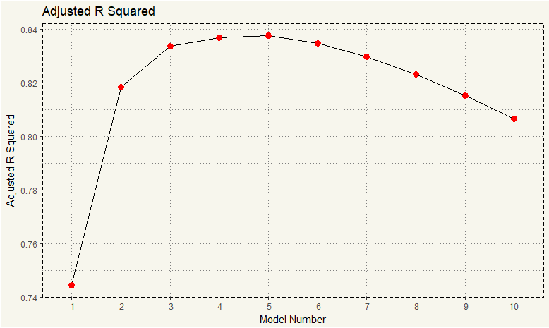
> stats$adjr2 [1] 0.7445939 0.8185189 0.8335561 0.8367919 0.8375334 0.8347177 0.8296261 0.8230390 0.8153314 [10] 0.8066423 |
Unfortunately, GGPLOT doesn’t work with regsubsets class. Therefore, we need some extra step for visualization.
|
1 2 3 4 5 6 7 8 9 10 11 12 13 14 |
##### Extracting Adjusted R-Squared ##### adjr2 <- stats$adjr2 number <- c(1:10) data <- data.frame(adjr2,cp,number) ##### Visualization ##### ggplot(data, aes(x = number, y = adjr2)) + geom_line() + geom_point(color = "red", size = 3) + theme_moma() + scale_x_discrete(limits = c(1:10)) + ylab("Adjusted R Squared") + xlab("Model Number") |

It seems like model number 5 is the best among the pack. We then can extract the coefficients by using coef() .
|
1 2 |
##### Extracting Coefficients ##### coef(bestsubsetselection, 5) |
|
1 2 3 |
> coef(bestsubsetselection, 5) (Intercept) disp hp wt qsec am 14.36190396 0.01123765 -0.02117055 -4.08433206 1.00689683 3.47045340 |
Unfortunately, regsubset is not compatible with the popular predict() function. Therefore to predict, we need to do a lot of data munging which we is covered in this post.
TL;DR In the era where we can collect data more than we can analyze, Best Subset Selection is good to know, but it could hardly be a preferred method.
