H1B or H-1B refers to a visa that an employer can apply for temporary workers. We will not discuss its usefulness or controversies that have been covered extensively by the media. On the contrary, we will look at the hard cold facts officially published by United States Department of Labor (DoL.) The data in this series is fiscal year 2017 and is released at the DoL web site (link) under “Disclosure Data” section.
But as usual, we need to load goodies.
|
1 2 3 4 5 6 7 8 9 10 11 12 13 14 15 16 17 |
##### Load Goodies ##### library(tidyverse) library(readxl) library(ggrepel) ##### Create Theme for GGPLOT2 ##### theme_moma <- function(base_size = 12, base_family = "Helvetica") { theme( plot.background = element_rect(fill = "#F7F6ED"), legend.key = element_rect(fill = "#F7F6ED"), legend.background = element_rect(fill = "#F7F6ED"), panel.background = element_rect(fill = "#F7F6ED"), panel.border = element_rect(colour = "black", fill = NA, linetype = "dashed"), panel.grid.minor = element_line(colour = "#7F7F7F", linetype = "dotted"), panel.grid.major = element_line(colour = "#7F7F7F", linetype = "dotted") ) } |
The DoL released the data in an Excel file format alongside an explanation in a PDF. Let’s load the data and take a look at its dimension.
|
1 2 3 4 5 |
##### Load Data ##### data <- read_xlsx('H-1B_Disclosure_Data_FY17.xlsx') ##### Dimension ##### dim(data) |
|
1 2 |
> dim(data) [1] 528146 40 |
Wow, 528,416 observations and 40 variables. I am sure that with that many variables, there are many interesting facts to discover. But as this is the first article in the series and is an introduction, we will only use only a few variables: CASE_STATUS, CASE_SUBMITTED, DECISION_DATE, VISA_CLASS, EMPLOYMENT_START_DATE, EMPLOYER_NAME, and TOTAL_WORKERS.
|
1 2 3 4 |
##### Data 2 ##### data2 <- select(data, CASE_STATUS, CASE_SUBMITTED, DECISION_DATE, VISA_CLASS, EMPLOYMENT_START_DATE, EMPLOYER_NAME, TOTAL_WORKERS) |
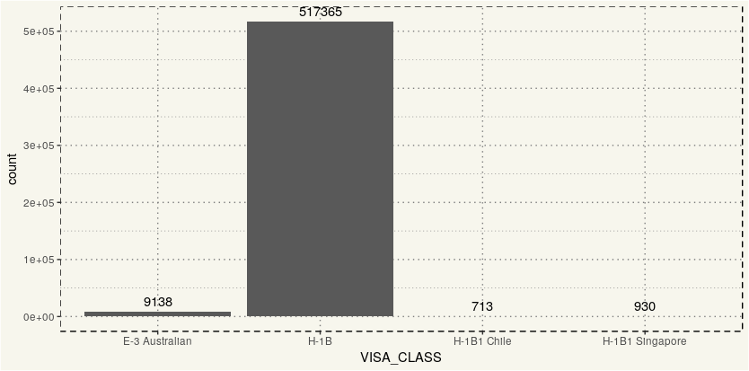
Let’s take a look at the VISA_CLASS first.
|
1 2 3 4 5 |
##### Visa Type ##### ggplot(data, aes(x = VISA_CLASS)) + geom_bar() + geom_text(stat='count',aes(label=..count..), vjust = -0.5) + theme_moma() |

The majority of the filing in the release is H1B visa which, I believe, applies to every nationality. The exception would be Chile, Singapore, and Australian in which they seem to have their specific visa type but is still considered non-immigrant visa. Since other visas are insignificant, there should be no need to analyze them separately.
Case Submitted
According to the explanation from DoL, the data is extracted from the Office of Foreign Labor Certification’s iCERT Visa Portal System where the decision date was between October 1, 2016, and June 30, 2017, inclusive.
It was an interesting criterion to use. If DoL uses the decision date, could there be a backlog in which an application submitted in 2012 but had just been approved/denied in 2017? We can use min() and max() on CASE_SUBMITTED.
|
1 2 3 4 |
##### CASE_SUBMITTED ##### data2 %>% summarise(Min = min(CASE_SUBMITTED), Max = max(CASE_SUBMITTED)) |
|
1 2 3 4 5 6 7 |
> data2 %>% + summarise(Min = min(CASE_SUBMITTED), + Max = max(CASE_SUBMITTED)) # A tibble: 1 x 2 Min Max <dttm> <dttm> 1 2011-03-23 2017-06-30 |
Mar 23, 2011? That’s 5 to 6 years of waiting for one single decision. 😐
Since the submitted date went back as far as six years, let’s create a time series chart.
|
1 2 3 4 5 6 7 8 9 10 11 12 13 14 15 16 17 |
##### CASE_SUBMITTED Plot ##### data2 %>% select(CASE_SUBMITTED) %>% arrange(CASE_SUBMITTED) %>% mutate(Month = format(CASE_SUBMITTED, "%m"), Year = format(CASE_SUBMITTED, "%y")) %>% select(Month, Year) %>% mutate(Count = n()) %>% ggplot(aes(x = Month, group = Count)) + geom_line(stat = "count") + theme_moma() + facet_grid(.~Year) + geom_point(stat = "count") + theme(axis.text.x = element_text(angle = 90, size = 7), panel.grid.minor = element_line(colour = "#F7F6ED", linetype = "dotted"), panel.grid.major = element_line(colour = "#F7F6ED", linetype = "dotted")) + geom_text_repel(stat='count',aes(label=..count..), size = 3) |
 It seems like most of the decision has been made relatively quick. But we can do better than that to find the average time it takes to get a final decision.
Processing Time
We can subtract CASE_SUBMITTED and DECISION_DATE to obtain the processing time.
|
1 2 3 4 |
##### Processing Time ##### data2 %>% mutate(Processing_Time = as.numeric((DECISION_DATE - CASE_SUBMITTED)/86400)) %>% select(Processing_Time) %>% summary() |
|
1 2 3 4 5 6 7 8 9 10 11 |
> data2 %>% + mutate(Processing_Time = as.numeric((DECISION_DATE - CASE_SUBMITTED)/86400)) %>% + select(Processing_Time, CASE_STATUS) %>% + summary() Processing_Time CASE_STATUS Min. : 0.00 Length:528146 1st Qu.: 6.00 Class :character Median : 6.00 Mode :character Mean : 31.21 3rd Qu.: 6.00 Max. :2214.00 |
They are fairly quick. The mean is only 31 days.
Employer
When it comes to H1B coverage, the media often cites tech giant such as Facebook and Microsoft. But are tech giants the only petitioners? Let’s do some simple count.
|
1 2 3 4 5 |
##### Employers ##### data %>% group_by(EMPLOYER_NAME) %>% summarise(count = n()) %>% arrange(desc(count)) |
|
1 2 3 4 5 6 7 8 9 10 11 12 13 14 15 16 17 18 |
> data %>% + group_by(EMPLOYER_NAME) %>% + summarise(count = n()) %>% + arrange(desc(count)) # A tibble: 65,132 x 2 EMPLOYER_NAME count <chr> <int> 1 INFOSYS LIMITED 17059 2 TATA CONSULTANCY SERVICES LIMITED 10806 3 CAPGEMINI AMERICA INC 8208 4 IBM INDIA PRIVATE LIMITED 7673 5 TECH MAHINDRA (AMERICAS),INC. 6903 6 ACCENTURE LLP 5573 7 DELOITTE CONSULTING LLP 5449 8 ERNST & YOUNG U.S. LLP 5143 9 GOOGLE INC. 4532 10 MICROSOFT CORPORATION 4042 # ... with 65,122 more rows |
Wow. There were 65,312 employers filed the H1B applications. By just eyeballing, it seems like these top 10 employees accounted for almost 100,000 submitted applications. What about the rest?
|
1 2 3 4 5 6 |
##### Summary ##### data %>% group_by(EMPLOYER_NAME) %>% summarise(count = n()) %>% arrange(desc(count)) %>% summary() |
|
1 2 3 4 5 6 7 8 9 10 11 12 13 14 |
> ##### Summary ##### > data %>% + group_by(EMPLOYER_NAME) %>% + summarise(count = n()) %>% + arrange(desc(count)) %>% + summary() EMPLOYER_NAME count Length:65132 Min. : 1.000 Class :character 1st Qu.: 1.000 Mode :character Median : 1.000 Mean : 8.109 3rd Qu.: 3.000 Max. :17059.000 |
Only three applications on average.
No. of Application VS. No. of Workers
When we apply for, say a new passport, we can only put one applicant in an application, right? So, how about an H1B application?
At first, I thought one application is for one worker. But it seems like I am wrong.
|
1 2 3 4 |
##### Worker VS Application ##### data %>% select(EMPLOYER_NAME, CASE_NUMBER, TOTAL_WORKERS, CASE_STATUS) %>% arrange(desc(TOTAL_WORKERS)) |
|
1 2 3 4 5 6 7 8 9 10 11 12 13 14 15 16 17 |
> data %>% + select(EMPLOYER_NAME, CASE_NUMBER, TOTAL_WORKERS, CASE_STATUS) %>% + arrange(desc(TOTAL_WORKERS)) # A tibble: 528,146 x 4 EMPLOYER_NAME CASE_NUMBER TOTAL_WORKERS CASE_STATUS <chr> <chr> <dbl> <chr> 1 DELOITTE CONSULTING LLP I-200-16307-558116 155 DENIED 2 APPLE INC. I-200-16319-287614 150 CERTIFIED 3 APPLE INC. I-200-16319-496930 150 CERTIFIED 4 APPLE INC. I-200-16319-541705 150 CERTIFIED 5 APPLE INC. I-200-16319-087529 150 CERTIFIED 6 APPLE INC. I-200-16319-172125 150 CERTIFIED 7 APPLE INC. I-200-16319-608407 150 CERTIFIED 8 APPLE INC. I-200-16319-401391 150 CERTIFIED 9 APPLE INC. I-200-16319-872666 150 CERTIFIED 10 APPLE INC. I-200-16319-217547 150 CERTIFIED # ... with 528,136 more rows |
Deloitte has submitted one application that has 155 workers. Apple, on the contrary, has filed multiple applications each with its unique case number with 150 workers each.
Consequently, the total number of workers whose employers applied an H1B visa for is not merely the sum of the case number. But the sum of the TOTAL_WORKERS by EMPLOYER_NAME.
Total Workers
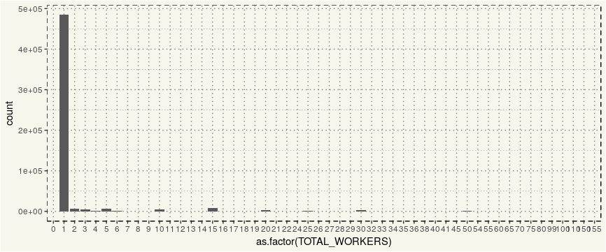
But, in general, how many workers are in an application?
|
1 2 3 4 5 |
##### How many workers in a application? ##### data2 %>% ggplot(aes(x = as.factor(TOTAL_WORKERS))) + geom_bar() + theme_moma() |

Oh okay. 90% of the application only has one worker. That makes sense. But the other 10% has more than one worker. Let’s modify the chart a bit.
|
1 2 3 4 5 6 7 8 |
##### Second Try ##### data2 %>% filter(TOTAL_WORKERS > 1) %>% ggplot(aes(x = as.factor(TOTAL_WORKERS))) + geom_bar() + theme_moma() + geom_text(stat='count', aes(label=..count..), size = 3, vjust = -0.5) + theme(axis.text.x = element_text(size = 7)) |

15 workers per applicant? But then I am not a legal expert. 🙂
Before we end this Overview post, how many of these applications have been approved?
|
1 2 3 4 5 6 |
##### Approval Rate ##### data2 %>% ggplot(aes(x = CASE_STATUS)) + geom_bar() + theme_moma() + geom_text(stat='count', aes(label=..count..), size = 3, vjust = -0.5) |

