There are crimes everywhere. But I believe full-grown adults’ concern regarding crime and the concerns for a family with young kids are different. Crimes such as kidnapping should affect children more than adults. Drugs should be a more significant concern to parents than to a couple.

Although websites such as Trulia and Zillow offer crime map, each crime is different. In this EDA, we will figure out what type of crime infest San Francisco Bay Area.

The datasets are published at Kaggle (Link.) Kaggle has separated the files into a train, and test sets as their purpose is to classify the type of crime. Since we are doing an EDA, we will combine them.

The data is already clean, so there is nothing much to do but just two simple things.

Okay, let’s see the data.

Almost 2 million observations of data. I would leave the “Address” variable alone. The “lon” and “lat” variables are particularly interesting to me.
As we will use it to for ggmap() , I want to check if there is an error.
First, we need to get San Francisco coordinates.

Okay, so SF’s lon and lats are -122.4194 and 37.77493.
Next, we need to check if the dataset has errors. As it is almost two million observations, I will not use geom_point but will use geom_boxplot()  instead.

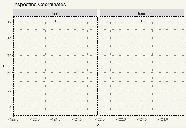
Oh, that is interesting. It is wrong. Longitude 90 is probably not even near San Francisco. Given that we have an outlier like this, it makes me want to see how the Y distributed in the dataset.

Okay, that is much better. It seems like the only error in this dataset is the data point. At this point, instead of creating a new dataset, I’ll use pipe operator for visualization.

Next, we need to download a map through ggmap() . ggmap()  can fetch data from Google, OSM, and Stamen with many map types.
In this case, I chose Stamen and terrain-lines for clear visualization.

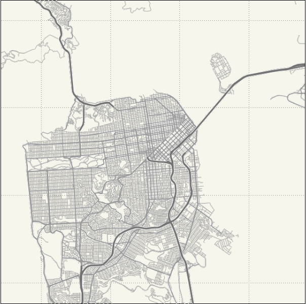
Ah, that’s beautiful. Since we already got the map, first of all, I want to see the aerial view of “PdDistrict.”

It is unfortunate that my laptop cannot handle plotting geom_point on 800K observations. So I used 100,000 observations to plot on ggmap. It is not perfect. But we now know where each district is.

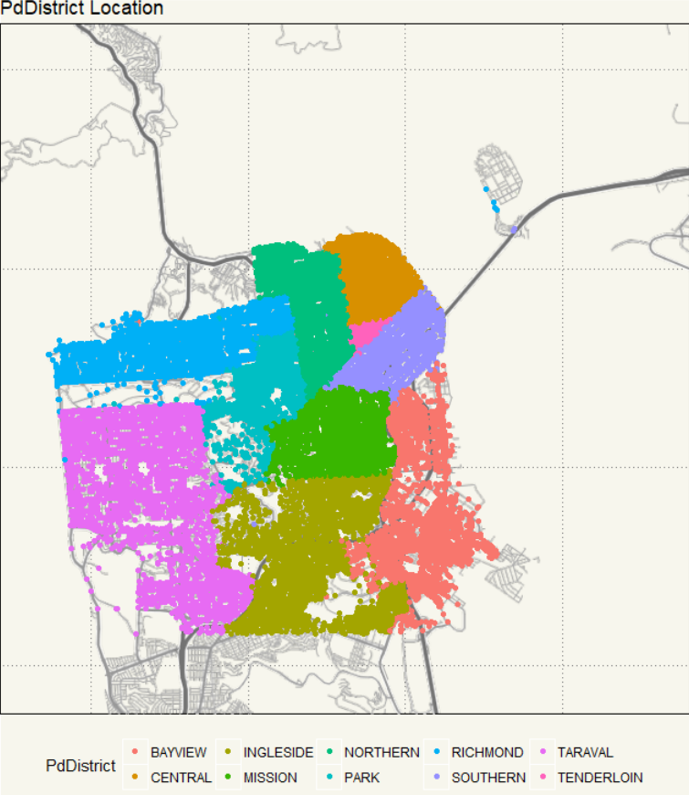
I guess that blue dots in the small island is the Alcatraz. So, let’s see what district is the most crime infested.

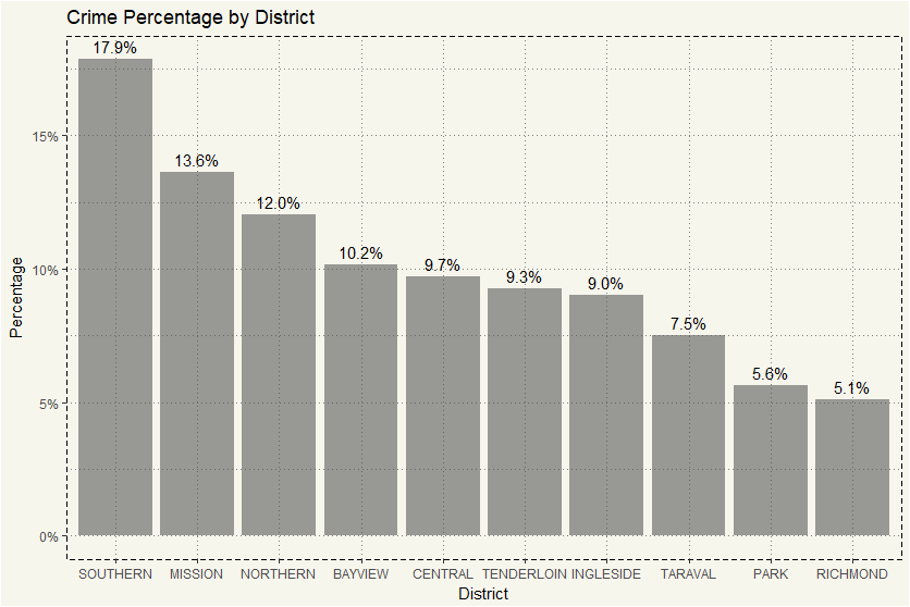
It seems like Southern is the most dangerous as it accounted for around 18% of the crime. At this point, we know that what district is dangerous. Let’s explore the type of crime in the train dataset.

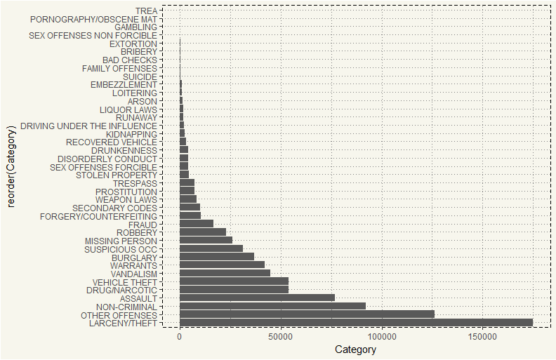
There are 39 types of crime in the dataset. As we assume that we are a family of four with two young kids, I think the offenses that are related to children are MISSING PERSON, KIDNAPPING, EXTORTION, and DRUG/NARCOTIC. We wouldn’t want our kids to get kidnapped,
or extorted, or to use drugs.

Instead of using pipe operator all the time, I’ll just create a new dataset for convenience and change the name a bit for easier visualization.

Now we are ready to see what are the areas we should avoid. But before we use a heat map to see the exact location, let’s see what type of crimes contributed the most in the areas.

Oh, it seems like San Francisco has some serious issue with drugs. Tenderloin appears to be a hotbed of crime as it has count way higher than the rest. I’m quite interested in Bayview. Let’s look at a different view.

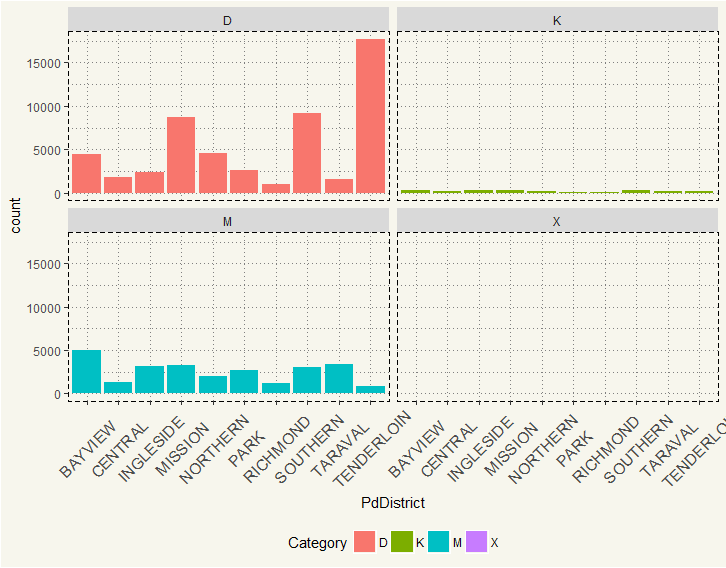So, that is interesting. Bayview seems to have particular a high number of missing person, while they rank 4th in term of all crime. Now, let’s use the heat map to determine where precisely these crimes occurred.

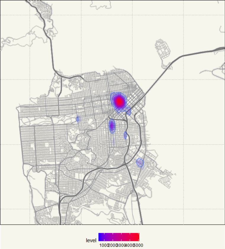
I have to say that it is interesting. Tenderloin seems to be such a hotbed of crime that the algorithm concentrated the density at Tenderloin. But this is not good for our visualization as we want to see where it is. Let’s try this workaround.

Okay, that’s better. But it is still too small, and if I were to put another layer, it would be too small to distinguish anyway. Let’s try another way.

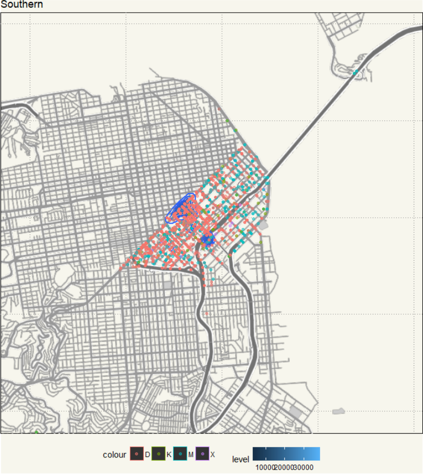
I feel like the area closed to Tenderloin is a hotbed of crime. They are just so concentrated in that area. So, Northeast San Francisco is not the place where we should go specifically Tenderloin and regions adjacent to Tenderloin. But if you could recall, you would notice that there are crimes in the entire Bay Area.

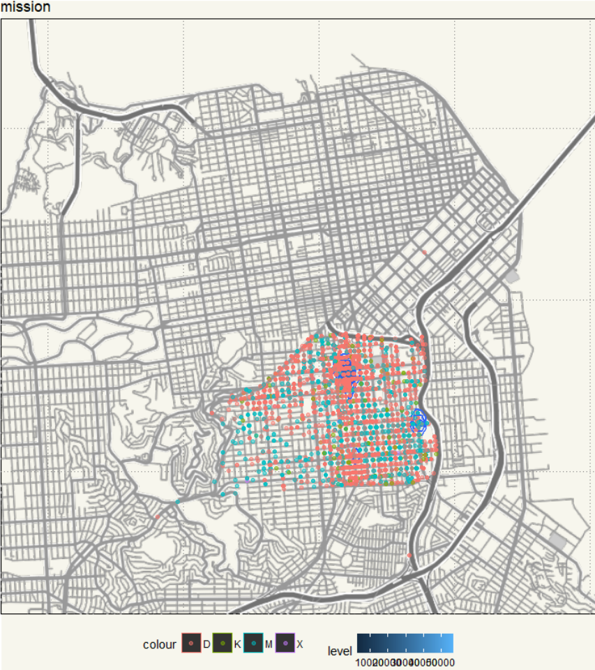
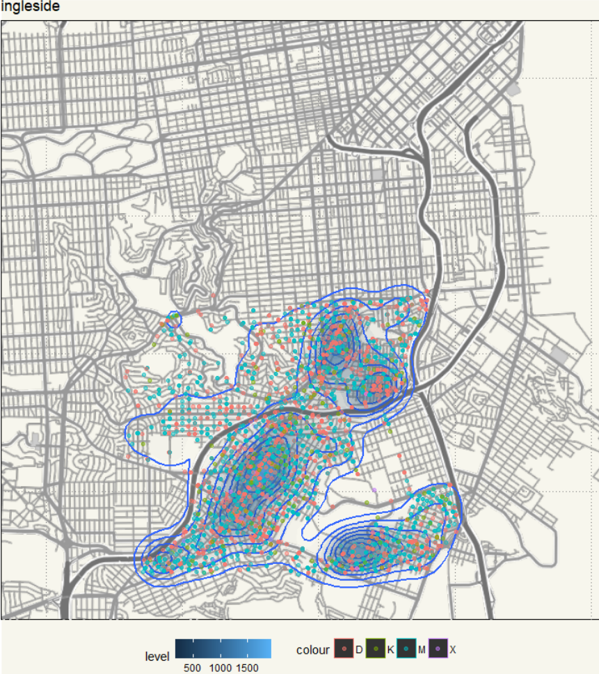
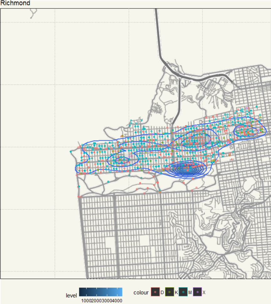
But not all in the above picture is covered by the stat_density. For example, crimes in Bayview mainly concentrated in just a specific area while the rest of the area has significantly much fewer occurrences. So, Tenderloin is off the list for sure as the entire area is infested with crime. But the others seem to have both safe and unsafe areas, let’s take a look at one by one.

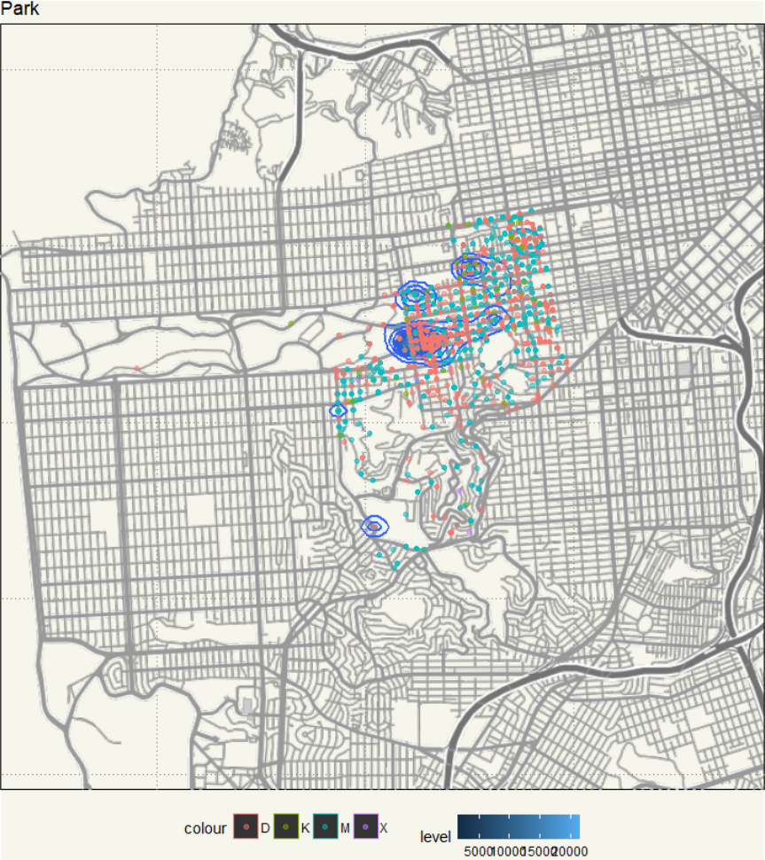
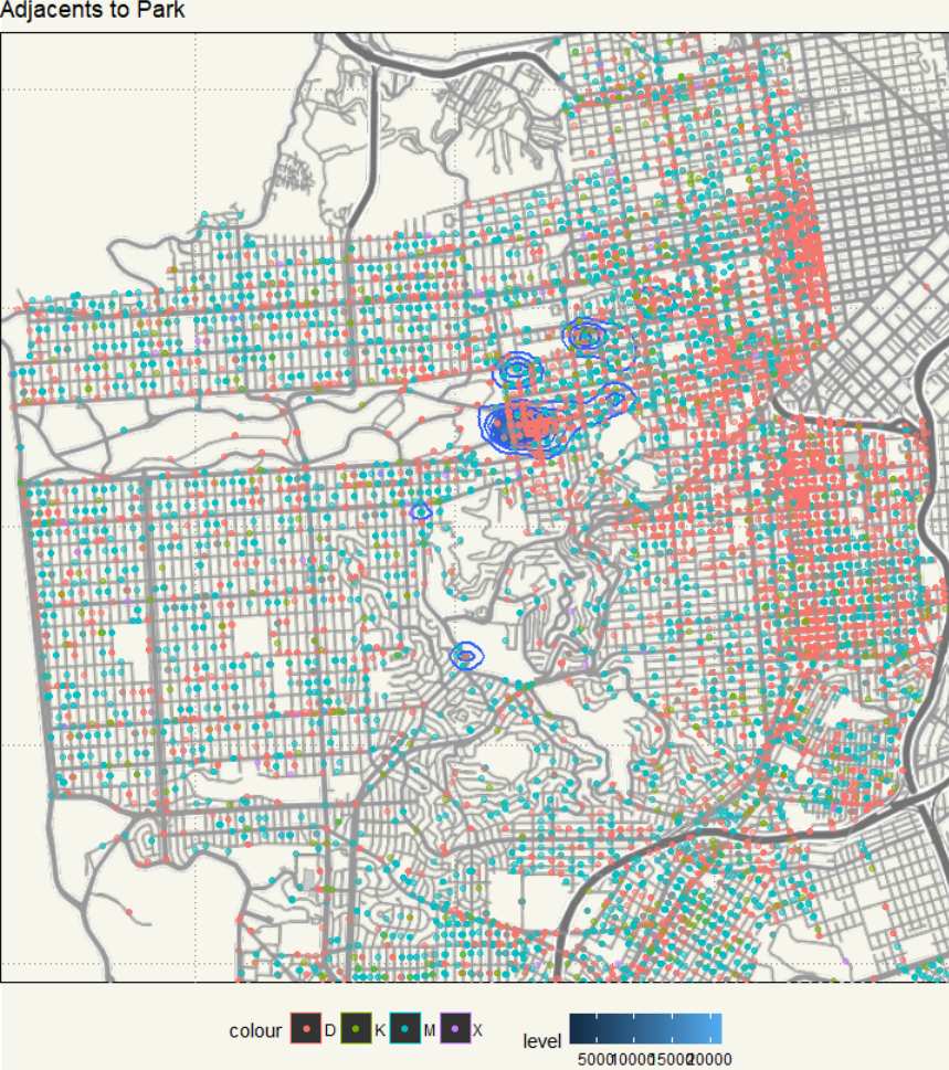
What about areas adjacent to Park and Mission.

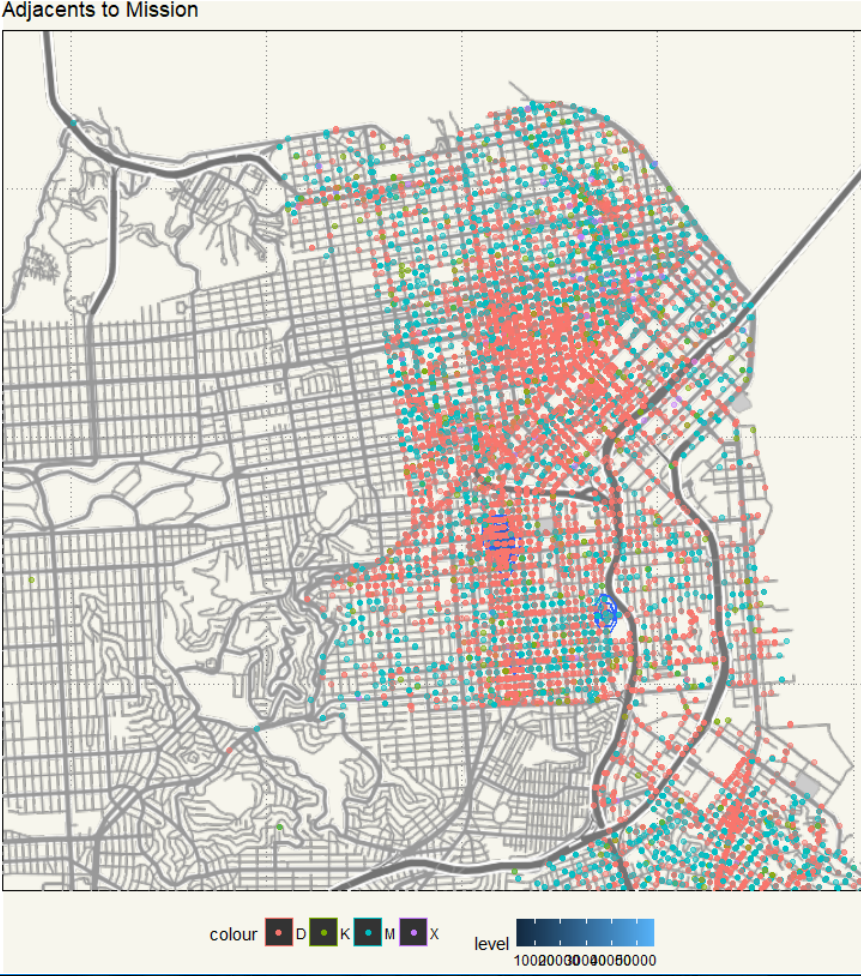
We now know what specific areas in each district we should settle down. Also, we should steer clear from the area adjacents to high crime districts.

A farewell note, I’d like to take a look at Kidnapping map.

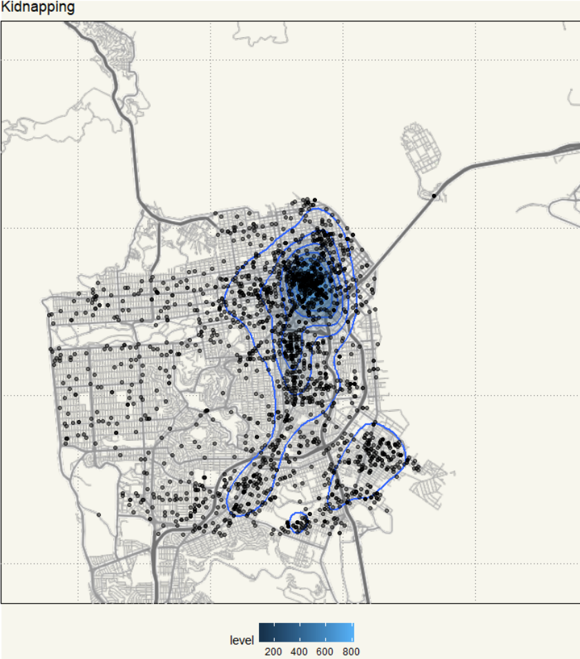
TL;DR Stay away from Tenderloin and its adjacent areas.