In this tutorial, we will examine an easy yet powerful technique called Decision Tree. There sure are many variations of the techniques from the most basic one (Classical Decision Trees) to an advanced cousin (Random Forest.) In this tutorial, we will focus on one variant of Decision Tree: Basic Decision Tree. We will utilize rpart library to train the Classical Decision Tree. So, let’s load the libraries!
|
1 2 3 4 |
##### Load Libraries ##### library(rpart) library(rattle) library(dplyr) |
We will use HR dataset to demonstrate the powerful yet simplistic Classical Decision Tree algorithm.
|
1 2 3 |
##### Load Data ##### data <- read.csv( "C:/Users/Data.csv", stringsAsFactors = T) |
But before we can use the algorithm, we need to prepare the data: one hot encoding for departments, and salary, and changing some names to be a little more self-explanatory.
|
1 2 3 4 5 6 7 8 9 10 11 12 13 14 15 16 17 18 19 20 |
##### Data Cleansing ##### ml <- data %>% rename(department = sales, accident = Work_accident, avg_mth_hrs = average_montly_hours, tenure = time_spend_company, promotions = promotion_last_5years) %>% mutate(dep_hr = ifelse(department == "hr", 1,0)) %>% mutate(dep_IT = ifelse(department == "IT", 1,0)) %>% mutate(dep_mngt = ifelse(department == "management", 1,0)) %>% mutate(dep_mkt = ifelse(department == "marketing", 1,0)) %>% mutate(dep_prod = ifelse(department == "product_mng", 1,0)) %>% mutate(dep_RandD = ifelse(department == "RandD", 1,0)) %>% mutate(dep_sales = ifelse(department == "sales", 1,0)) %>% mutate(dep_sup = ifelse(department == "support", 1,0)) %>% mutate(dep_tech = ifelse(department == "technical", 1,0)) %>% mutate(sal_med = ifelse(salary == "medium",1,0)) %>% mutate(sal_high = ifelse(salary == "high",1,0)) %>% #removing original variables select(-department, -salary) |
As usual, we will split the data into train and test sets.
|
1 2 3 4 5 6 7 |
##### Split the Dataset ##### size <- floor(0.75*nrow(ml)) set.seed(999) train_index <- sample(seq_len(nrow(ml)), size = size) train <- ml[train_index,] test <- ml[-train_indexx,] |
75% of the data or 11,249 observations (rows) will be a train set, while the rest (25% or 3,750) will be a test set. Now we are ready, let’s build the Classical Decision Tree model!
|
1 2 3 4 |
##### Classical Tree - Train ##### classical.tree <- rpart(left ~ ., data = train, method = "class", parms = list(split = "information"), control = rpart.control(xval = 15, cp = 0)) |
There are three critical parameters in the code: xval , cp , and split .
- Xval controls the number of cross-validation (the more, the better.)
- CP (Complexity Parameter) controls the split (the more, the stringent the split.) CP default value is 0.01. If the tree split does not improve the fit by cp, then it will not split. So, when I set it to 0, I just simply want the algorithm to split as much as they’d like.
- Split controls how a tree gets split. The rpart algorithm supports many options. I generally use either Gini or Information Gain. In all honesty, I try everything — as it is super easy by just changing the word — and pick the best one according to situations 😝.
Next, we will plot some chart.

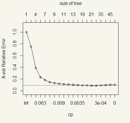
The error drops significantly at the fourth split and slows down until there is hardly any improvement after the ninth split.
Let’s see the numbers.
|
1 2 |
##### CP Table ##### classical.tree$cptable |
|
1 2 3 4 5 6 7 8 9 10 11 12 13 14 15 16 17 18 19 20 21 22 |
> classical.tree$cptable CP nsplit rel error xerror xstd 1 2.488839e-01 0 1.00000000 1.00000000 0.016826379 2 1.811756e-01 1 0.75111607 0.75111607 0.015141984 3 7.793899e-02 3 0.38876488 0.38876488 0.011453999 4 5.171131e-02 5 0.23288690 0.23288690 0.009045332 5 3.422619e-02 6 0.18117560 0.18154762 0.008038037 6 1.711310e-02 7 0.14694940 0.14732143 0.007271705 7 1.041667e-02 8 0.12983631 0.13020833 0.006850797 8 7.812500e-03 9 0.11941964 0.12090774 0.006609161 9 5.952381e-03 10 0.11160714 0.11458333 0.006438988 10 5.208333e-03 11 0.10565476 0.10863095 0.006274094 11 3.720238e-03 12 0.10044643 0.10305060 0.006115001 12 3.348214e-03 14 0.09300595 0.09821429 0.005973320 13 1.488095e-03 15 0.08965774 0.09114583 0.005759332 14 1.116071e-03 16 0.08816964 0.09151786 0.005770811 15 5.208333e-04 20 0.08370536 0.08705357 0.005631369 16 3.720238e-04 25 0.08110119 0.08816964 0.005666580 17 2.480159e-04 34 0.07738095 0.09188988 0.005782266 18 1.594388e-04 37 0.07663690 0.09709821 0.005940095 19 9.300595e-05 44 0.07552083 0.10081845 0.006050065 20 0.000000e+00 54 0.07366071 0.10230655 0.006093441 |
After we let the algorithm loose, there are 54 splits! Whoa, okay, well, that is way too much. Surely, it is the time to prune. Now is the time when things can be entirely subjective. Maybe your client doesn’t want the tree to be more than 10, or your boss wants the most thorough tree possible regardless of the complexity. If there is no mandate from an Ivory Tower resident, I personally use the \(cp\) from lowest split whose error range falls in this formula \(xerror \pm xstd\) applied to the highest split. In this case, the range is \(0.102\pm 0.006\) or 0.096 to 0.1084. Looking at the result, the 11th attempt or 12 split has \(xerror\) fall within the range with the least split. Then we will use its \(cp\) in the prune() function.
|
1 2 |
##### Let's Prune ##### classical.pruned <- prune(classical.tree, cp = 3.720238e-03 ) |
Now it’s time to plot the tree.
|
1 2 |
#### Plotting the Pruned Tree ##### fancyRpartPlot(classical.pruned,tweak =1.3) |

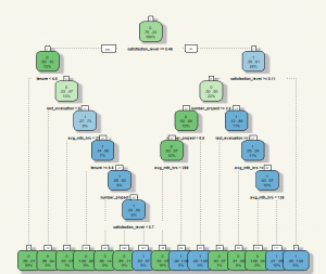
My apology for the font size. It was quite a pain to adjust the look-and-feel of the Decision Tree. From the chart, we can see that the algorithm mainly uses average hours work, satisfaction level, and a number of projects. With this information, we can hard code the prediction using ifelse() and apply to the test set. But why would we do that as we have predict() function? 😝
|
1 2 |
##### Predict ##### classical.predict <- predict(classical.pruned, test, type = "class") |
Next, we evaluate the prediction.
|
1 2 |
##### Model Evaluation ##### table(classical.predict,test$left) |
|
1 2 3 4 5 |
> table(classical.predict,test$left) classical.predict 0 1 0 2850 68 1 17 815 |
Oh, that is even better than Logistic Regression. The accuracy is \(\frac{2850+815}{(2850+815+68+17)}\) or 97.7%.
Despite the excellent performance, if you look closely, you will see that the algorithm didn’t use a categorical variable at all (e.g., department, salary.) This is the exhaustive search bias. The issue is addressed in other Decision Tree iterations, one of which is Conditional Inference Tree.
TL:DR; In this example, Classical Decision Tree could predict with 97.7% accuracy rate despite its super easy to implement algorithm. However, this is not its best yet… there are far more advanced cousins: Conditional Inference Tree, and Random Forest. 🙂
